NASA Exoplanets

Data Modeling

Exoplanets are planets outside our solar system. Is the exoplanet Confirmed?

Above is an artist's rendering of NASA's Kepler Space Telescope in search of them.NASA documents 4,164 and counting "Confirmed" exoplanets discovered so far and thousands of other "Candidate" planets. Below is the process I used to create data models using telescope observations to predict a planet's status.

As of writing this there are 4,164 "confirmed" exoplanets. The other "candidate" planets require more study to be confirmed. The discovery method most often successful is the transit method as the exoplanet passes in between it's star and the telescope. The dimming of the light from that star can then be measured and the orbit studied.

I chose the Planetary Systems Alpha release dataset which is essentially all the planetary data combined. The data consists of 26,336 rows and 118 columns. Out of 118 columns some just had too many missing values, others were not helpful to predict if it's a confirmed planet, or the column variable was hard to understand. After all, understanding the data can be important to not leak training data to testing data.

Links to follow along:

The first thing was to explore the data columns. Initially I had 118 different data columns so I narrowed it down to 25. Out of these 22 were numeric data types and 3 were categorical types. I'm first going to describe the numeric columns of planetary data.

Numeric Columns

Heatmap

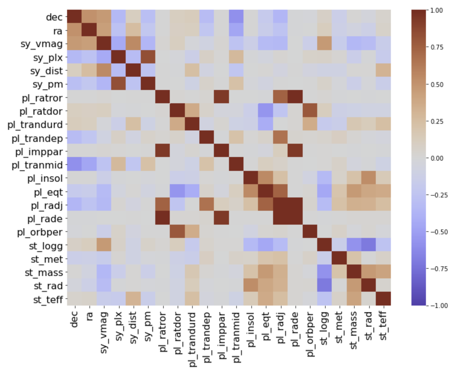
The heatmap shows any correlations between the columns.

Each column shows up once on the left margin and again at the bottom.
The diagonal line is created because of course the column is highly correlated with itself.
"dec" and "ra" are the location cooridinates of the planets.
The columns beginning with "sy" refer to the planetary systems. Notice how they're grouped together and create a pattern.
The columns begining with "pl" refer to the exoplanets. "pl_radj" and "pl_rade" refer to the radii or radiuses of the planets measured in units of Jupiters and Earths. There are definitely some correlations among these.
The columns begining with "st" refer to the star the exoplanet orbits. Notice how these create a pattern.

"pl_eqt" is the planet's temperature.

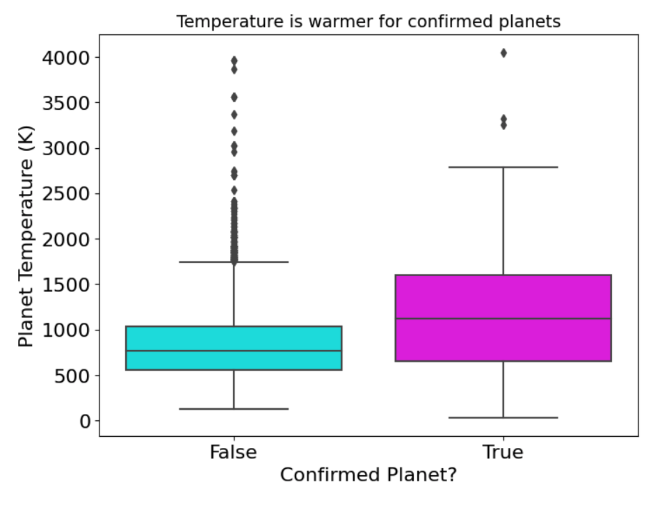
This boxplot shows Confirmed planets in magenta have on average a warmer temperature.

"pl_orbper" is orbit time in days and "pl_ratdor" is a ratio of distance from the planet to it's star.

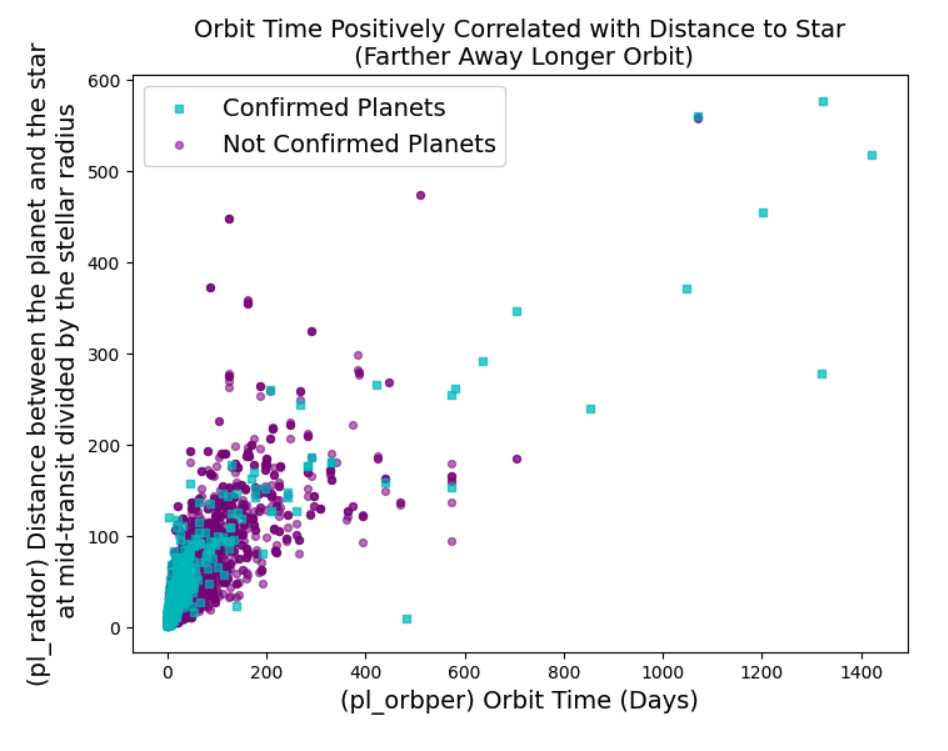
This scatterplot shows Confirmed planets in teal are more closely grouped with shorter orbit times. Overall, the farther away a planet is the longer time it takes to orbit the star.

"pl_trandep" is flux caused by transit of the planet and "pl_radj" is the planet radius measured in Jupiter units.

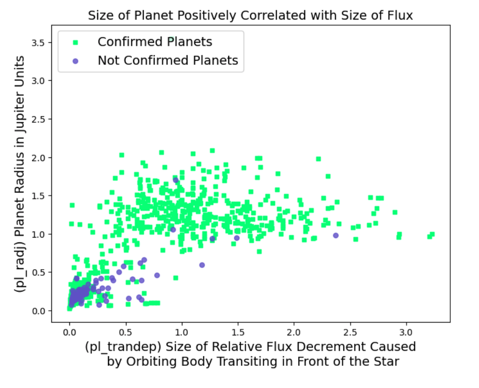
This scatterplot shows Confirmed planets in green cause more flux or change in brightness of the star by their transit. Overall, larger planets cause more flux.

"pl_trandurd" is the transit duration in hours. "pl_rade" is the planet radius in earth units. "st_mass" is the stellar mass (Click to enlarge).

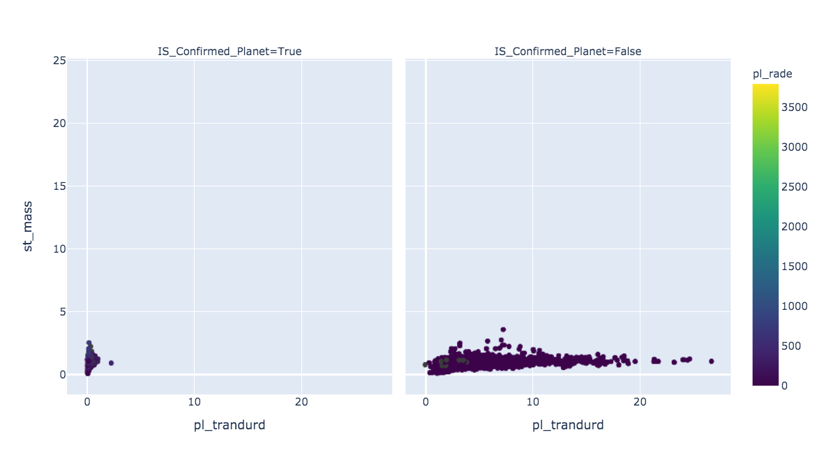
The transit duration in hours will be a very important predictor (see feature importances) because it's longer for planets that have NOT been confirmed. The stellar masses on the y axis shows little difference. Planet radii on the color bar shows some differences especially if you zoom in. To zoom in click on the graph and there's a tool bar at the top right to zoom and a pan tool to see different areas.

"pl_imppar" is the distance of planet to star. "pl_ratror" is the ratio of planet to star radius.

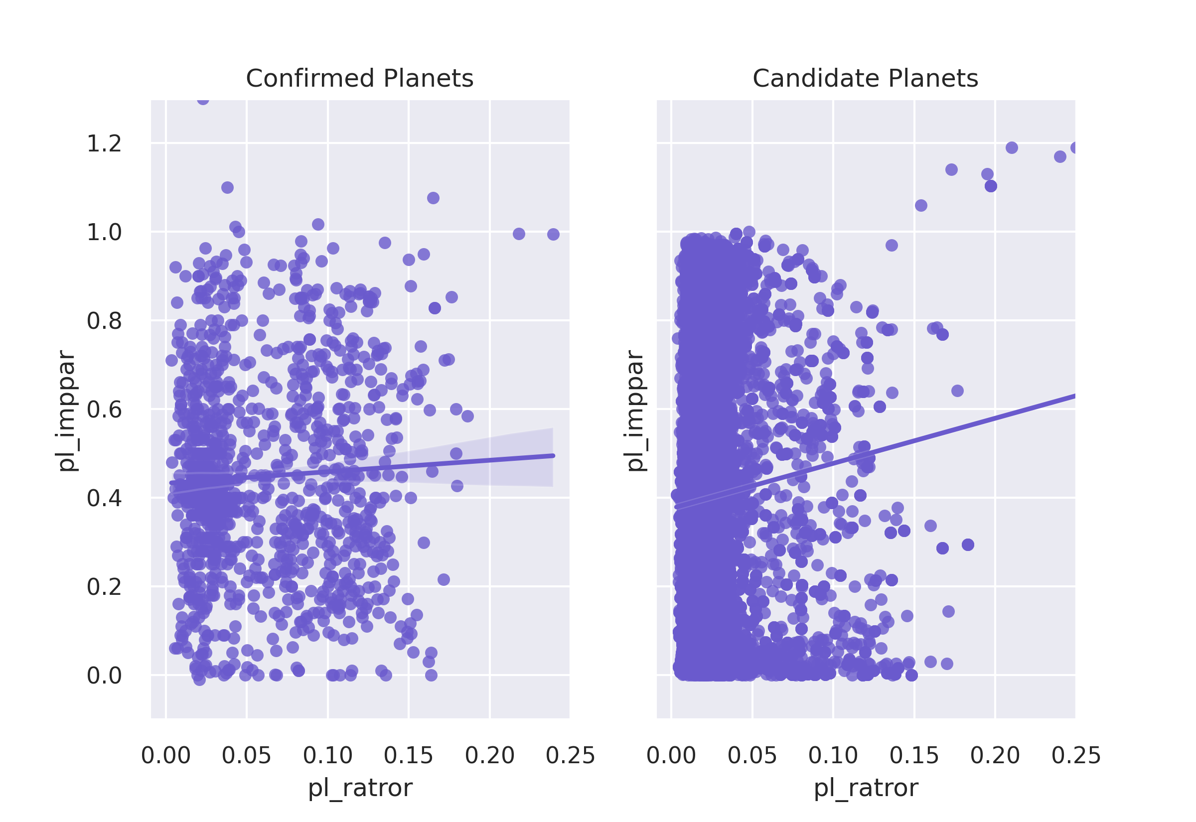
This linear regression scatter plot shows Confirmed and Candidate planets are grouped differently. The linear trendlines are different too.

"pl_ratdor" is a ratio of distance from the planet to it's star. "pl_eqt" is the planet's temperature.

As the distance increases (X axis) the planet temperature decreases (y axis). So distance and temperature are correlated by if the planet is cooler it must be farther away from it's star. Overall, there's less distance from planet to it's star for confirmed planets.

"ra" is the planet's longitude east and west coordinates."dec" is the planet's latitude north and south coordinates."st_mass" is the stellar mass (Click to enlarge).

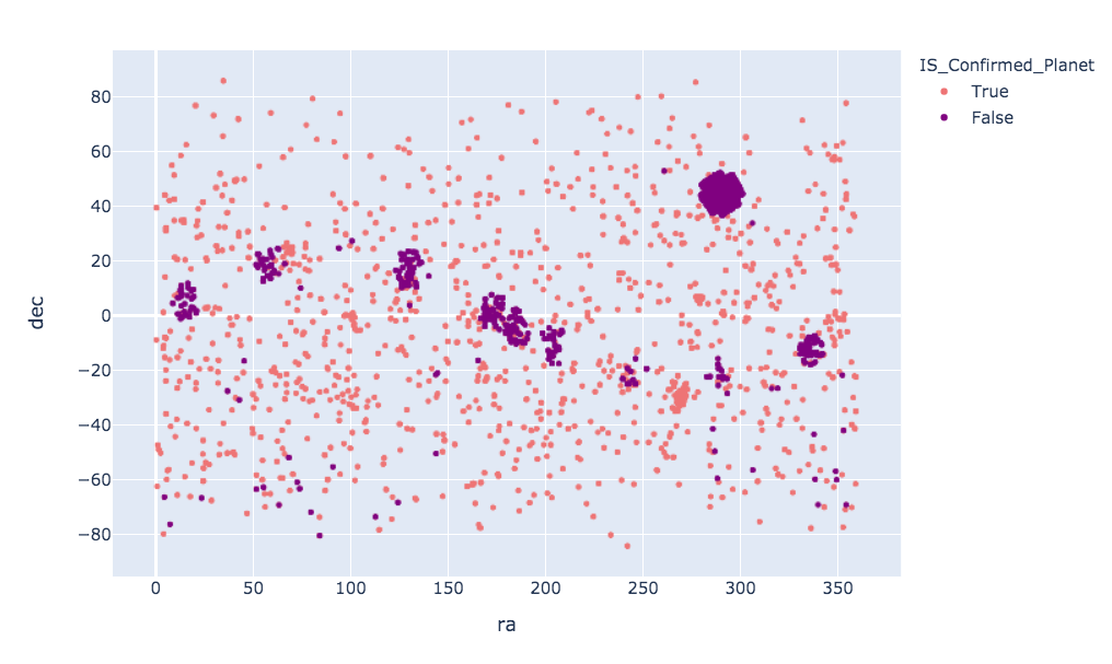
Right ascension and declination are the equivalent of longitude and latitude for an object's celestial coordinates. Here it's easy to see all the confirmed and candidate planets. Kepler's original mission is focused on the top right darker square shape. Kepler in it's original operational condition no longer works the same but is now functioning as K2. K2's discoveries go across in a swooped line.

Categorical Columns

"discoverymethod" is obviously how the planet was discovered.

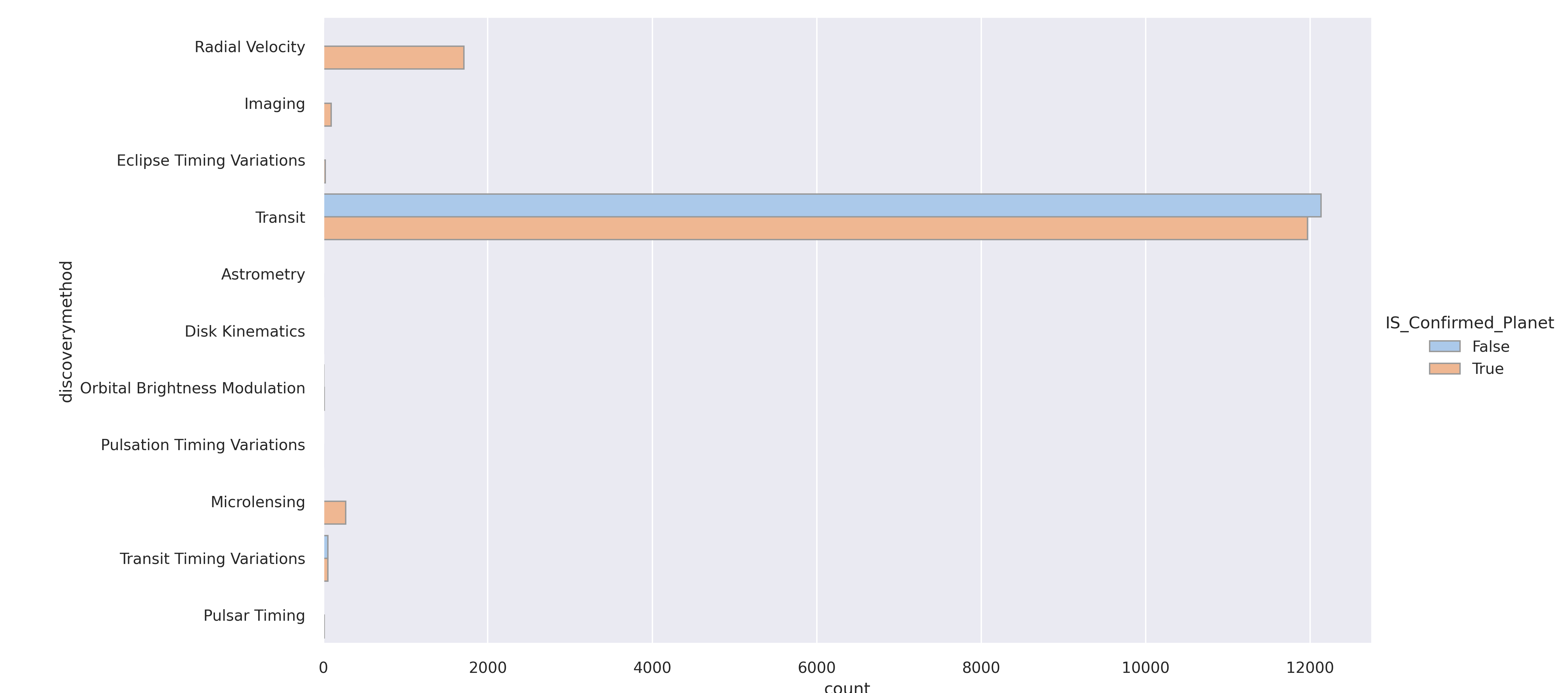
Transit is clearly the most common and is how Kepler made it's discoveries. Radial Velocity is when the star wobbles slightly because of the gravitational pull of its orbiting exoplanet. Radial Velocity was used to discover all confirmed planets which is a good predictor.

"disc_locale" is of course where the planet was discovered.

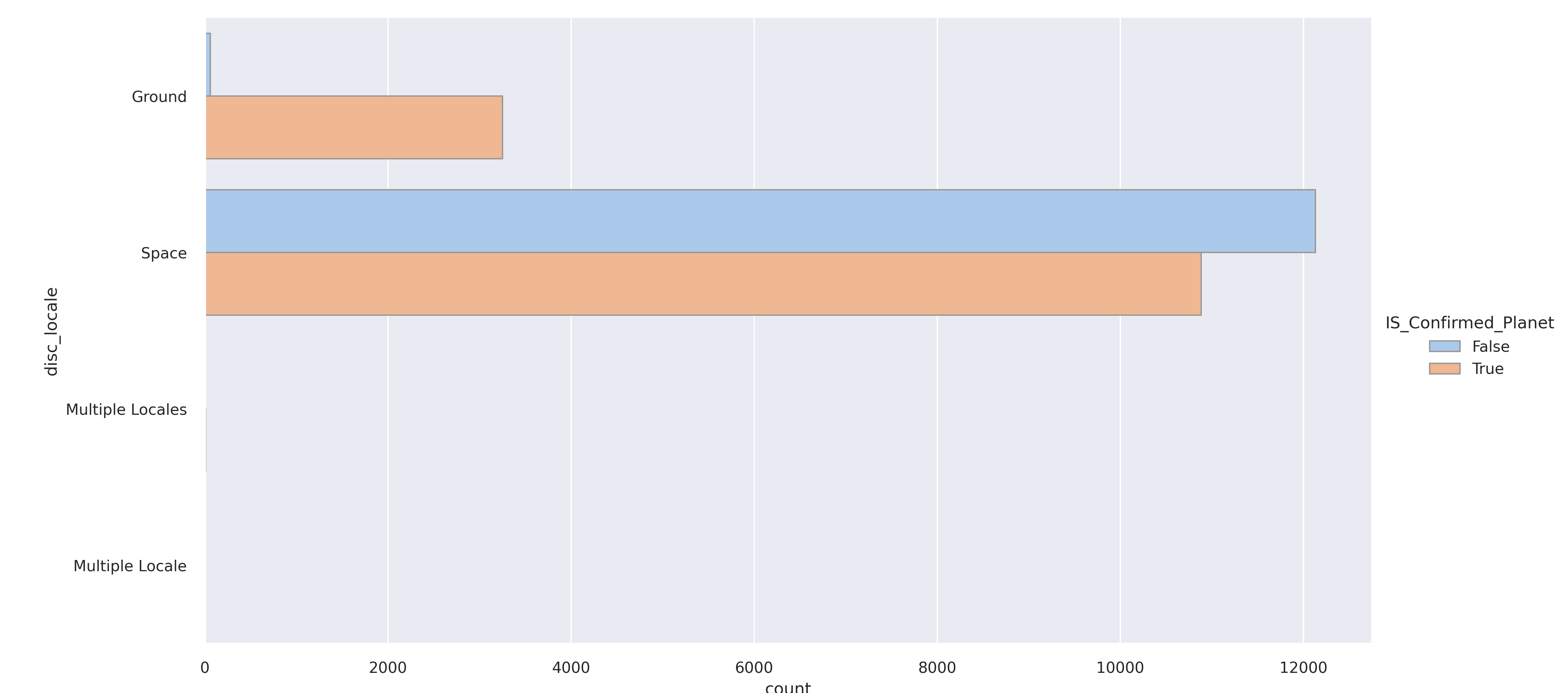
Planets discovered on the ground are more likely to be confirmed planets. The clear majority of the rest of planets were discovered in space by Kepler like telescopes that can reach farther and see better images.

"st_metratio" is the star's metal ratio.

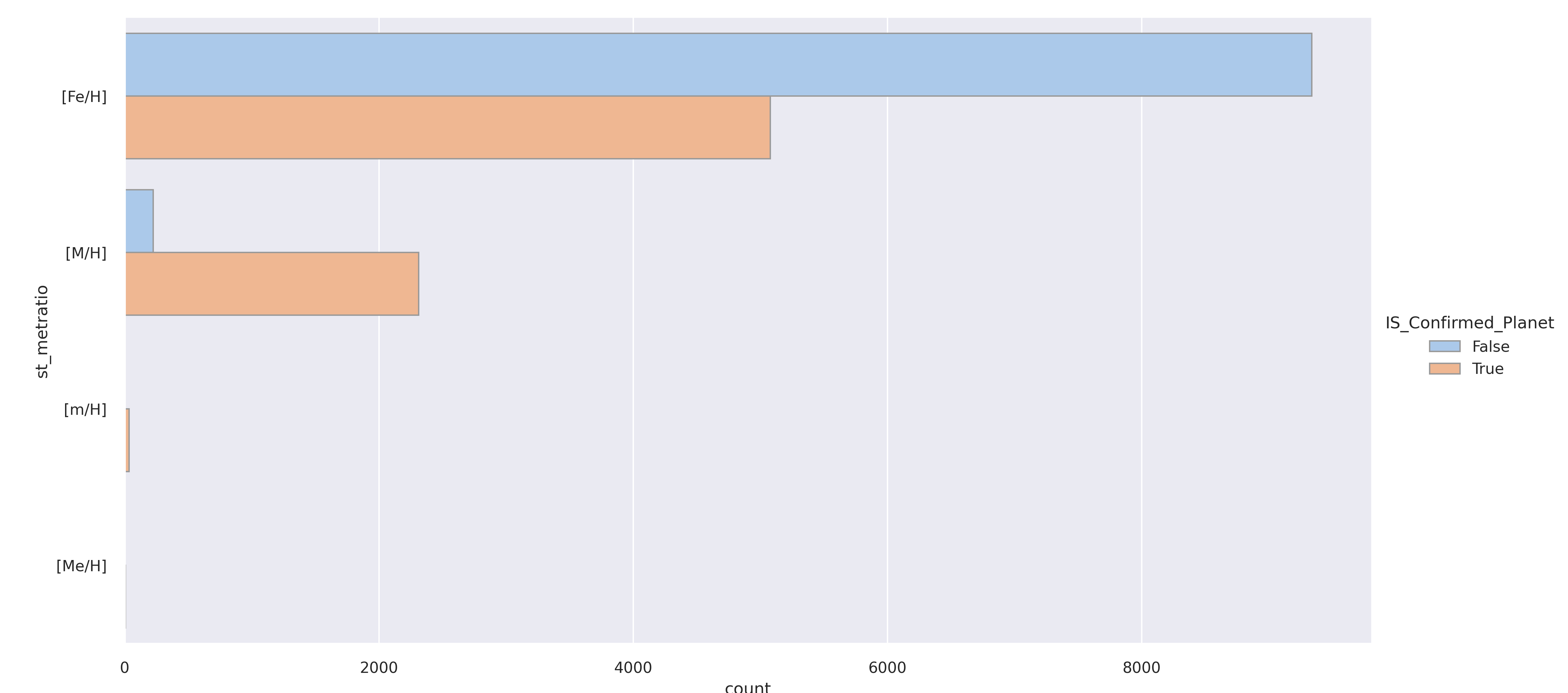
Ratio for the Metallicity Value [Fe/H] denotes an iron abundance, [M/H] refers to a general metal content. So there are more candidate unconfirmed planets in the iron column and more confirmed planets in the general metal column. These two features will likely be important predictors.

Predicative Model Making - Is the exoplanet confirmed or not?

Baseline & Logistic Regression (LR) Model

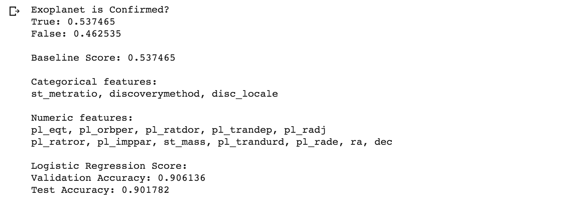
Using the numeric columns: "pl_eqt", "pl_orbper", "pl_ratdor", "pl_trandep", "pl_radj", "pl_ratror", "pl_imppar", "st_mass", "pl_trandurd", "pl_rade", "ra", "dec" and the categorical columns "st_metratio", "discoverymethod", "disc_locale"

The best guess would be True because True's have a 53.7% majority.
The first predictive model using Logistic Regression improved the best guess prediction to a 90.2% certainty.

Confirm Logistic Regression Score

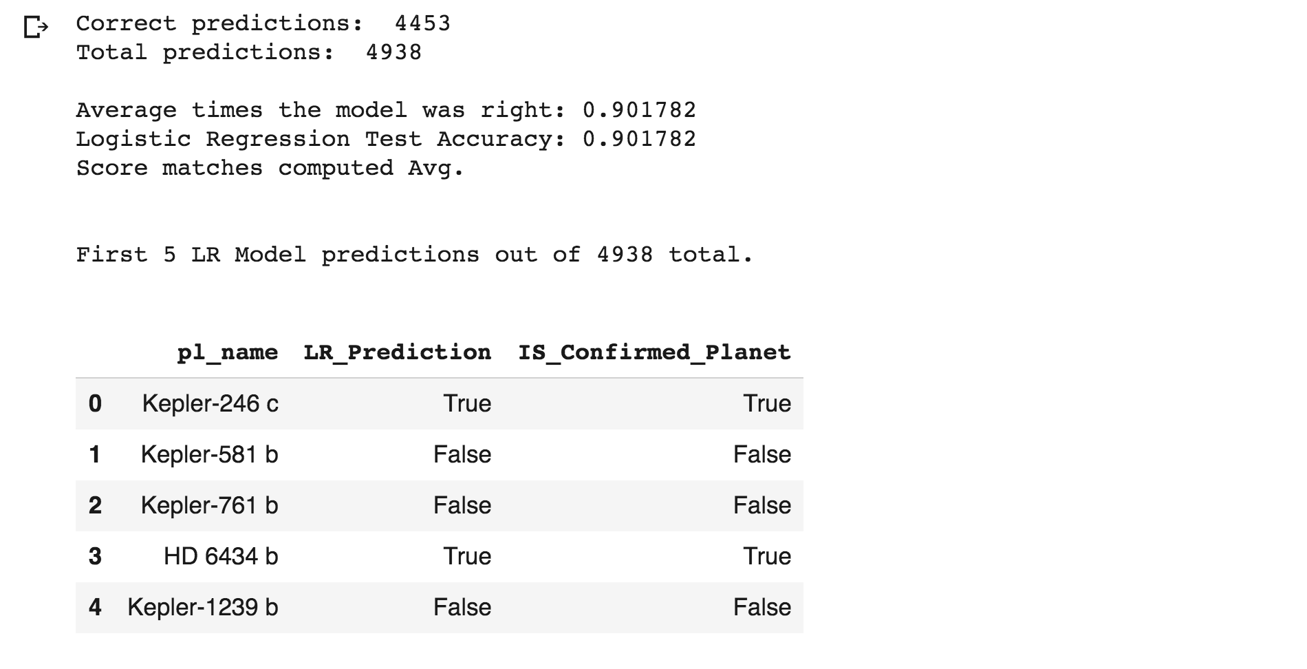
There were a total of 4,938 predictions made. 4,453 were right and 485 were wrong giving the model score a 90.2%
The model's accuracy score was verified by dividing the number of correct predictions by the total number of predictions and everything matched.
The first 5 LR Model predictions which all happened to be correct can be seen below along with the planet names.
So only a little less than 10% of the predictions were wrong.

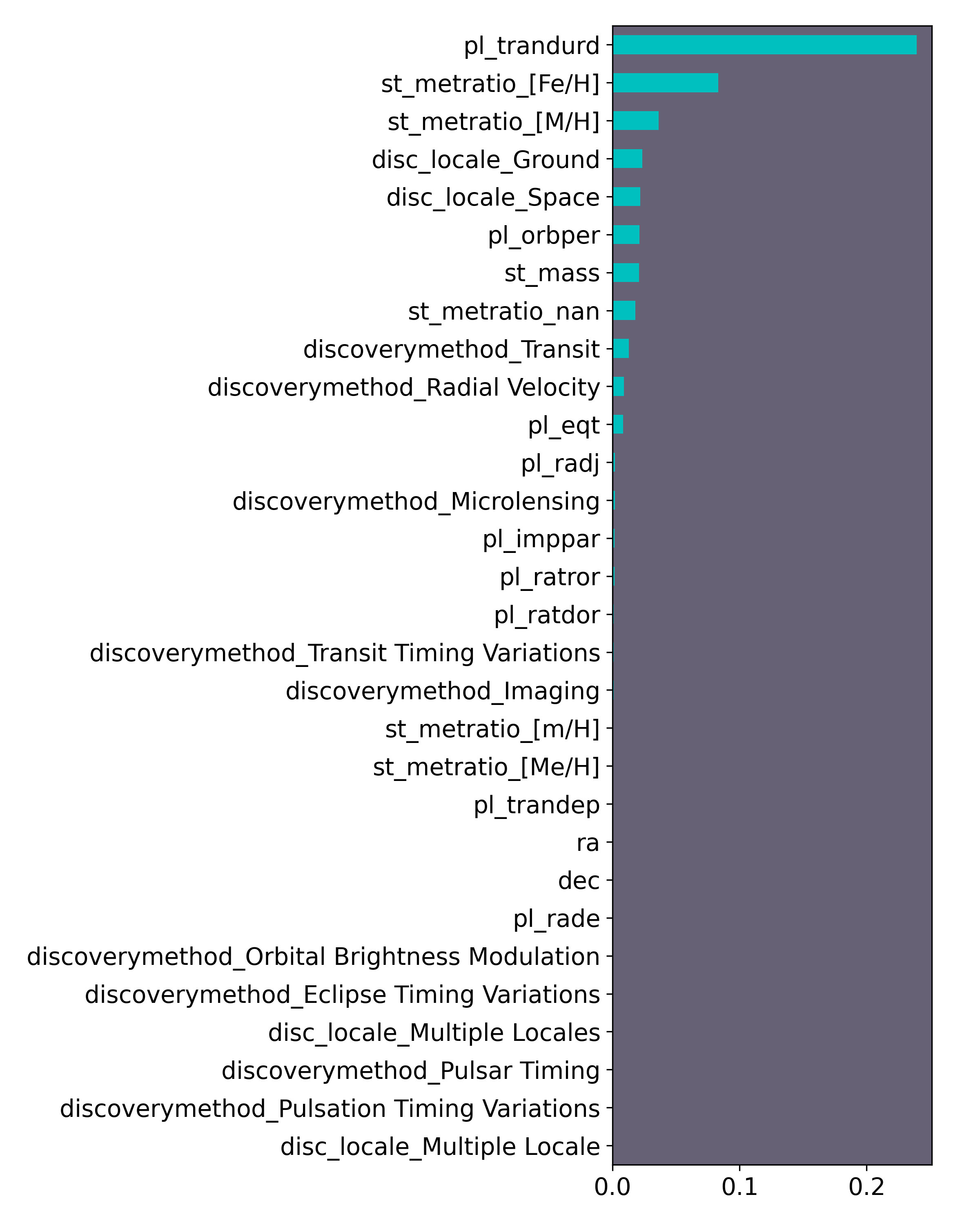
LR feature importances (permuted)

Permuted means the feature's importance was double checked by shuffling it, then finding it's impact on model accuracy.
Obviously the features with the most green were the most important to the model's success.
There are a lot of features here that aren't helping the model so let's run it again using the best features.

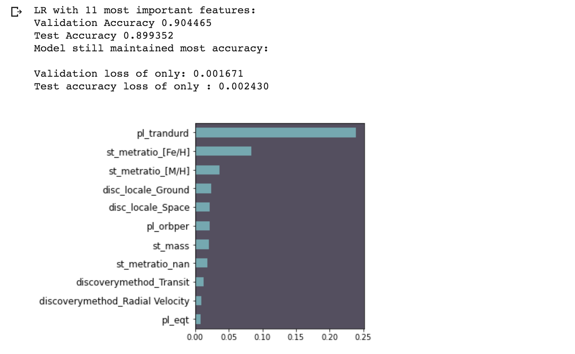
LR with top features

With the 11 most important features above the model test accuracy was still great at 90% (rounded up).
Out of all the 30 features we really only needed 11 to create a predictive model.
In a Kaggle Competition we would keep all features with an importance above 0.0% to get every small bit of improvement in the model score. With this model the feature importance cut off was 0.005. The prediction score only lost 0.2% accuracy, down from 90.2% to 90%.

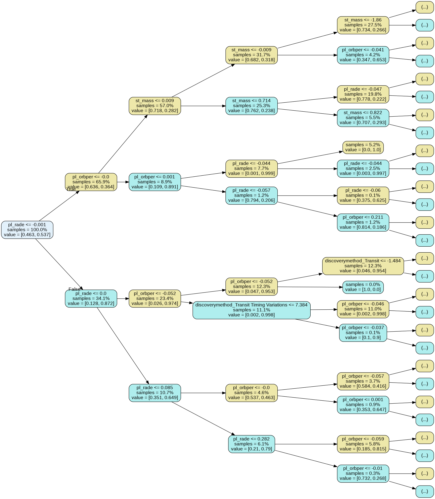
Decision Tree Model

Using only these columns:"pl_rade", "pl_orbper", "st_mass", "discoverymethod"

The Decision Tree Model and the following models use only 4 columns.
With Decision Trees to avoid overfitting the training data max_depth is a parameter that should be defined. For the next visual it was set to 4.
This helps the model keep generalized for the unpredictable test set and new data.
Here is a visual understanding how the DT set decision points to make predictions. The True's can be visualized in the color yellow and the False's in the color blue-green.

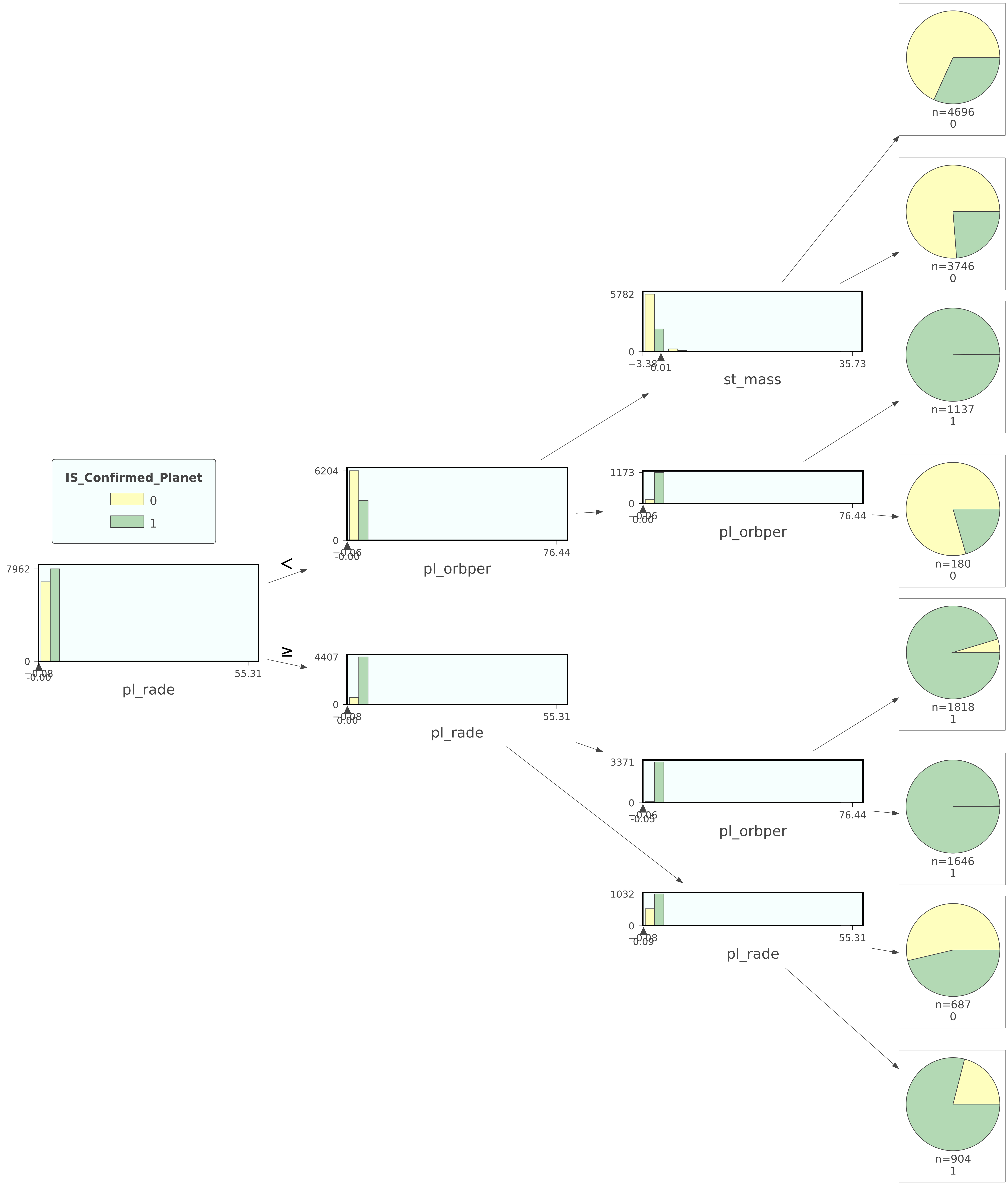
Another Decision Tree Visual using the Dtreeviz Library (link) with the max_depth set to 3. It uses a pie chart visual to make the model easier to interpret.
Here the root node is "pl_rade" meaning the decision process starts here. If it is less than it goes to the next decision which is "pl_orbper" (the majority here were candidate 0). If it is greater than or equal to it goes to the next decision which is "pl_rade" (the majority of these were confirmed 1). This process continues until the decision classifies that planet as confirmed or not confirmed.

The Decision Tree Model score was first ran with a max_depth kept at it's default of None and had an accuracy of 79.1% on the test set.
It was then ran again with a max_depth of 3 and it didn't overfit the training data but it did lose a very small amount of test accuracy. Down from 79.1% to 78.6%.
79.1% is used below in the final summary & comparison.

Random Forest Model

Continuing with the same columns: "pl_rade", "pl_orbper", "st_mass", "discoverymethod"

The Random Forest Model is just a bunch of Decision Trees ran using the feature columns. Then the most popular prediction (confirmed or not) is used in the final. Kind of like getting multiple opinions or estimates on a car before fixing it instead of just going with the first estimate.
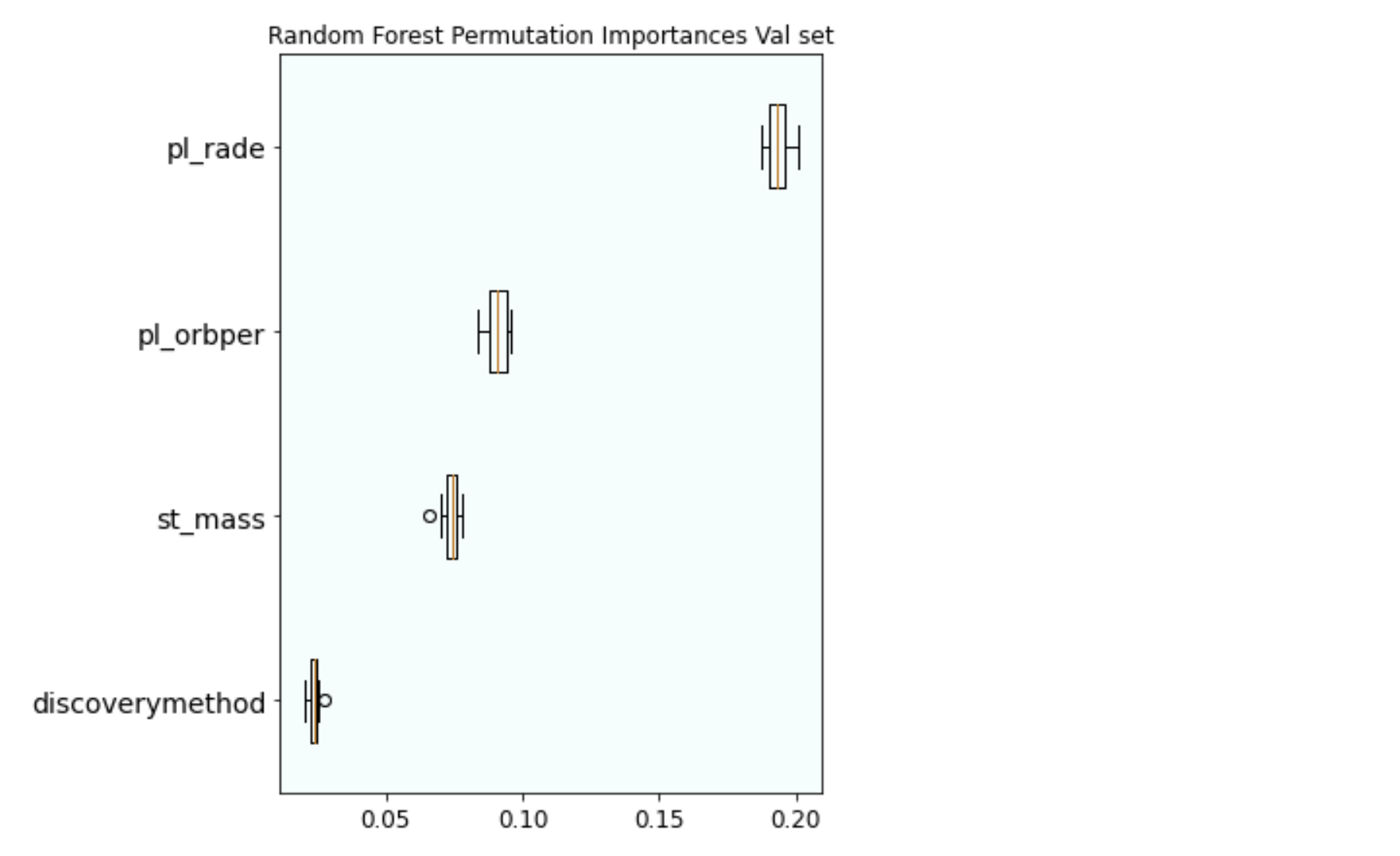
The Random Forest Model feature importances.

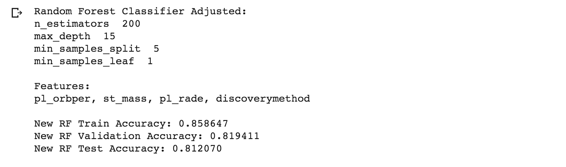
Random Forest Model with adjusted parameters improves the test score to 81.2%.

The default of 100 n_estimators was changed to 200.
The default of None max_depth was changed to 15.
The default of 2 min_samples_split was changed to 5.
The default of 1 min_samles_leaf was the only parameter not changed and left at 1.
New test score of 81.2%.

Cross Validation Model and Summary

Same columns: "pl_rade", "pl_orbper", "st_mass", "discoverymethod"

In a Cross Validation Model small subsets of the data are validated across the training data.
The RandomizedSearchCV method chose random parameters from our specified list.
n_iter was put at 20 which was the number of times a new set of random parameters were tried.
cv was put at 5 meaning 5 train / val splits were done for each one of the 20 different sets of parameters. Finally, out of those 20 model settings the model with the best average prediction score accuracy on it's 5 splits was used for the test set.
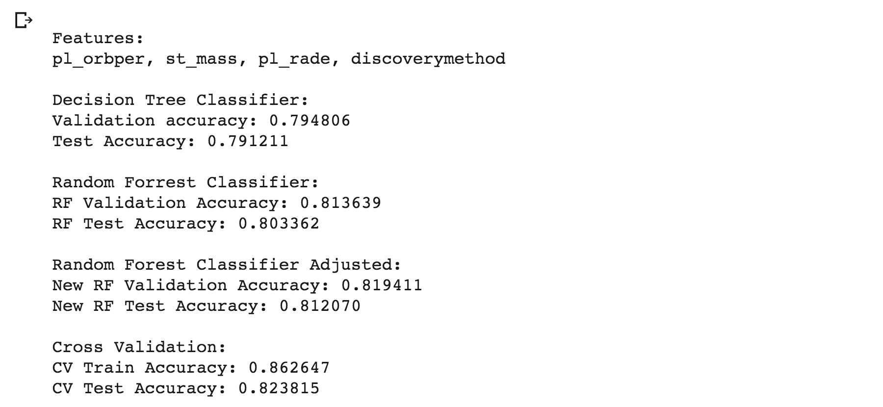
Cross Validation had the best test score of 82.4% as seen below.
Out of all the other models it took the longest to run about 5 minutes.
Beginning with The Decision Tree, next The Random Forest, RF Adjusted, and finally The CV each model saw an improvement in test accuracy.

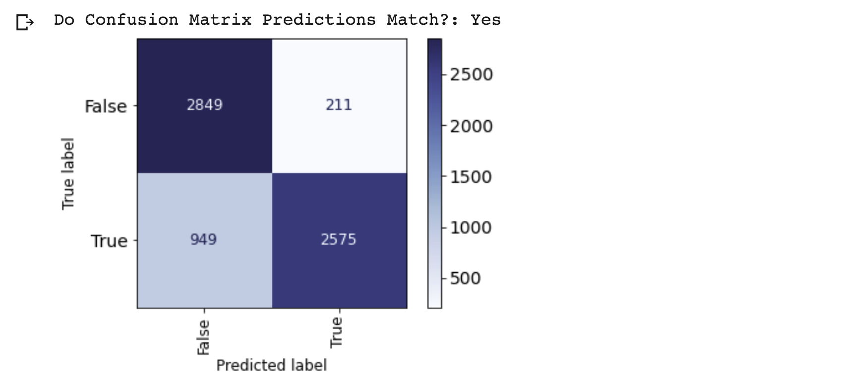
The Confusion Matrix of the Cross Validation Model just shows the correct True & False predictions match and the totals are correct.
The CV Model's False predictions were correct 2,849 times. It's True predictions were correct 2,575 times. It was wrong a total of 1,160 times (found by adding 949 plus 211).
We can verify our accuracy score by dividing the correct predictions by the total predictions. The result is 82.4% which matches above.

Conclusion

This was a big dataset so it was really helpful to reduce the number of columns to better understand them. Beginning with the Logistic Regression Model more columns were used to initially train the model. Starting with 12 numeric and 3 categorical columns. The 3 categorical columns would later become 18 features after being seperately encoded. For instance, the column "st_metratio" became 5 seperate features. The column "discoverymethod" became 9 and "disc_locale" would become 4 to create 18. Those added to the 12 numeric features created a total of 30 features. The model was trained and then again with only 11 of the most important features.

Using all the same features for the Decision Tree Model it was able to fit itself to a 99.3% accuracy. So using 3 numeric columns and 1 categorical column (12 features after encoding) it gave the Decision Tree and other Models more of a challenge. After running a Random Forest and changing the parameters the score improved. The best predictive model score with those 4 columns or 12 features came from a Cross Validation Model. For this project I learned a lot about predictive data modeling through the interesting topic of exoplanets. Thank you for following along.